Understanding Generalization Performance for Deep Classifiers

Posted by Rahul Pandey, Angeela Acharya, Junxiang (Will) Wang and Jomana Bashatah. Presented by Zhengyang Fan, Zhenlong Jiang and Di Zhang.

---

Classification in Machine Learning

A general problem of classification in machine learning can be defined as predicting an outcome y from some set Y of possible outcomes, on the basis of some observation x from a feature space X.

Mathematically, we can define a classification problem as to find a map $f: X \rightarrow Y$ based on $n$ observations $(x_1, y_1), ..., (x_n, y_n)$ such that $f(x)$ is a good prediction of $y$ for a new observation $(x, y)$.

To measure the success of the map $f: X \rightarrow Y$, we generally define loss function. Low loss function score implies better classification model.

Deep Learning in Classification

Most recent approach to solve classification problem is to use Deep Learning. Deep Learning uses deep networks, which are statistically deep compositions of non-linear functions.

$$f = f_L \circ f_{L_1} \circ ... \circ f_{1}$$

There are various non-learning function, which has been used in deep learning. Some of the popular ones are sigmoid function and ReLu (Rectified Linear Unit) function.

Sigmoid

$f_i \rightarrow \sigma(W_ix)$, where

$$\sigma(v_i) = \frac{1}{1+e^{-v_i}}$$

ReLu

$f_i \rightarrow \sigma(W_ix)$, where

$$\sigma(v_i) = max\{0,v_i\}$$

Deep Learning and Generalization

Deep Networks Classifiers generally perform much better than the traditional machine learning. That means their function map has a very low loss function score not only on training data, but on test data as well. However, classifiers in deep learning are heavily parameterized due to the complex nature of deep networks. The reason for its optimal performance despite overfitting is because of the size of the function space, which is large enough to interpolate data points.

In this blog, we will investigate the generalization of deep networks and compare its performance.

Before jumping on generalization, let’s talk about the probabilistic assumption of a deep learning model.

Given a probability distribution $\mathbb{P}$ on $X \times Y$, we define a function $f$ such that the risk $R(f)$ is minimized.

Risk is defined as

$$R(f) = \mathbb{E}l(f(X), Y)$$

where $\mathbb{E}$ is expectation and $l$ is loss over all $X \times Y$ i.i.d. pairs.

NOTE i.i.d. $\rightarrow$ independent and identically distributed random variables

Now, to measure the richness of function $\mathcal{F}$ over all $X \times Y$ i.i.d. pairs, we define Rademacher Complexity.

Rademacher Complexity

As stated above, Rademacher Complexity are used to find the richness of the learnt function in ML. Now, given a function $\mathcal {F}$, the Rademacher Complexity is $\mathbb{E}{\left \| R_n \right \|}_{\mathcal{F}}$, where the empirical process $R_n$ is defined as

$$R_n(f) = \frac{1}{n}\sum^{n}_{i=1} \epsilon_if(X_i)$$

where $\epsilon_i$ are Rademacher random variables, which are i.i.d. uniform on $\{-1, 1\}$

Rademacher Complexity for Deep Networks

Two-layer Neural Network

We define the training function $\mathcal{F_{B,d}}$ of a two-layer neural network as

$$\mathcal{F}_{B,d,L} = \left \{ x \rightarrow \sum^{k}_{i=1} w_i \sigma \left ( v_i^T x \right ) : {\left \| w \right \|}_1 \leq B, {\left \| v_i \right \|}_1 \leq B, k \geq 1 \right \}$$

where $B > 0$ and the non-linear function $\sigma : \mathbb{R} \rightarrow [0,1]$ satisfies the 1-Lipschitz condition, $\| \sigma(a) - \sigma(b) \| \leq \| a - b \|$ and $\sigma(0) = 0$.

Suppose that the distribution is such that ${\left \| X \right \|}_{\infty} \leq 1$, then

$$\mathbb{E} {\left \| R_n \right \|}_{\mathcal{F}_{B, d}} \leq 4B^2 \sqrt{\frac{2\log{2d}}{n}}$$

where $d$ is the dimension of the input space $X$

Hence, we can get the upper bound on a feed forward neural network, which is a function of dimension d. This implies that deep neural network can be generalized for better optimization, which will save a lot of computation and better out-of-sample performance over the test data.

Also, one interesting observation is that we can’t use sigmoid as a non linear function. It is because for sigmoid, $\sigma(0) \neq 0$, which changes the convergence property of the optimization network.

Experiments

We will be observing the effect of generalization on different deep networks. For this, we have observed the CIFAR 10 data, which is a famous object detection dataset in computer vision that has images from 10 distinct classes. We have observed the effect of 3 deep neural networks: Inception, AlexNet, and 1X512 Multi-layer perceptron.

We inspected the behavior of neural networks trained on varying level of label corruptions (we intentionally change the correct labels of training set). By corrupting the labels, we want to observe if the network can actually generalize well on training data with all the wrong labels.

We observed two parameters: time to overfit and test error. Figure 1. shows both the results distributed over the degree of label corruptions.

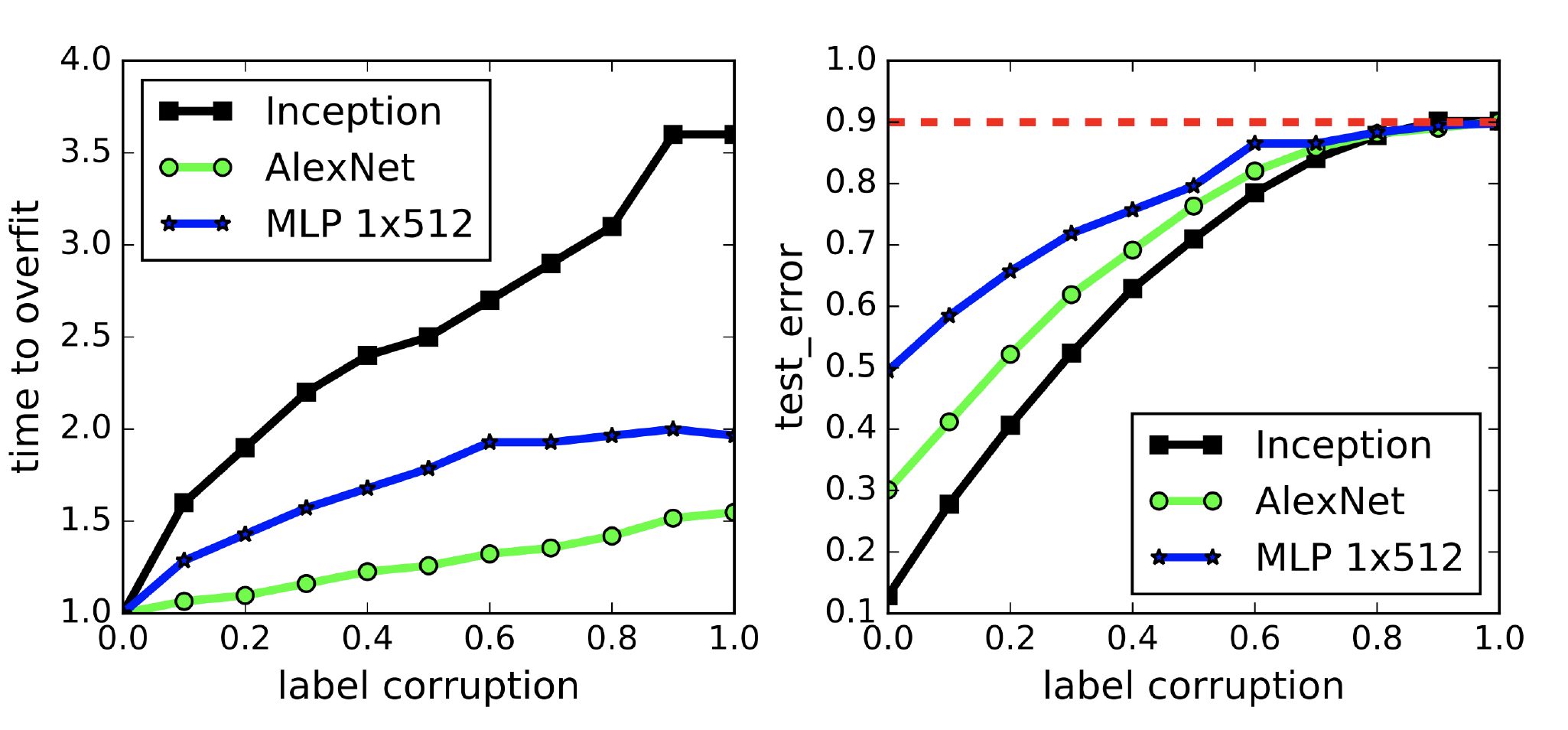
Fig 1. a.) convergence slowdown b.) generalization error growth

One point to remember was that the network fit to the corrupted training set perfectly for all the degree of label corruptions. From the first figure, we can see that the time taken for convergence of neural network is not linear w.r.t. degree of label corruptions. In fact, as we increase the corrupted label, sometimes it actually took almost similar or even less time to converge for some cases.

The second figure depicts the error on test set after convergence on the corrupted training data. Since we are fully overfitting the model with the corrupted training data, the test errors are same as generalization errors. We can see once we fully corrupted the training set, the generalization errors converges to 90%, which is the exact performance of random guessing of CIFAR 10.

Hence, to summarize

1. Deep network can easily fit random variables.
2. It has still good out of sample performance, even in sample error is 0 (100% overfit)
3. This is true for random label problems

Hence, we can conclude that all the models were generalized perfectly, even with the addition of random noise to the network’s parameters.

Unique observations on Kernal Ridge Regression

We just observed that the generalization of model is necessary. However, sometimes the mechanism for good out-of-sample performance can be achieved with higher interpolation (overfitting) over in-sample training data.

Consider the following example of a Kernal ridge regression on MNIST data shown in Figure 2. We have observed the log error of out of sample digit pairs over different lambda value of regularization parameters. Regularization is used for generalization and minimize the in sample interpolation.

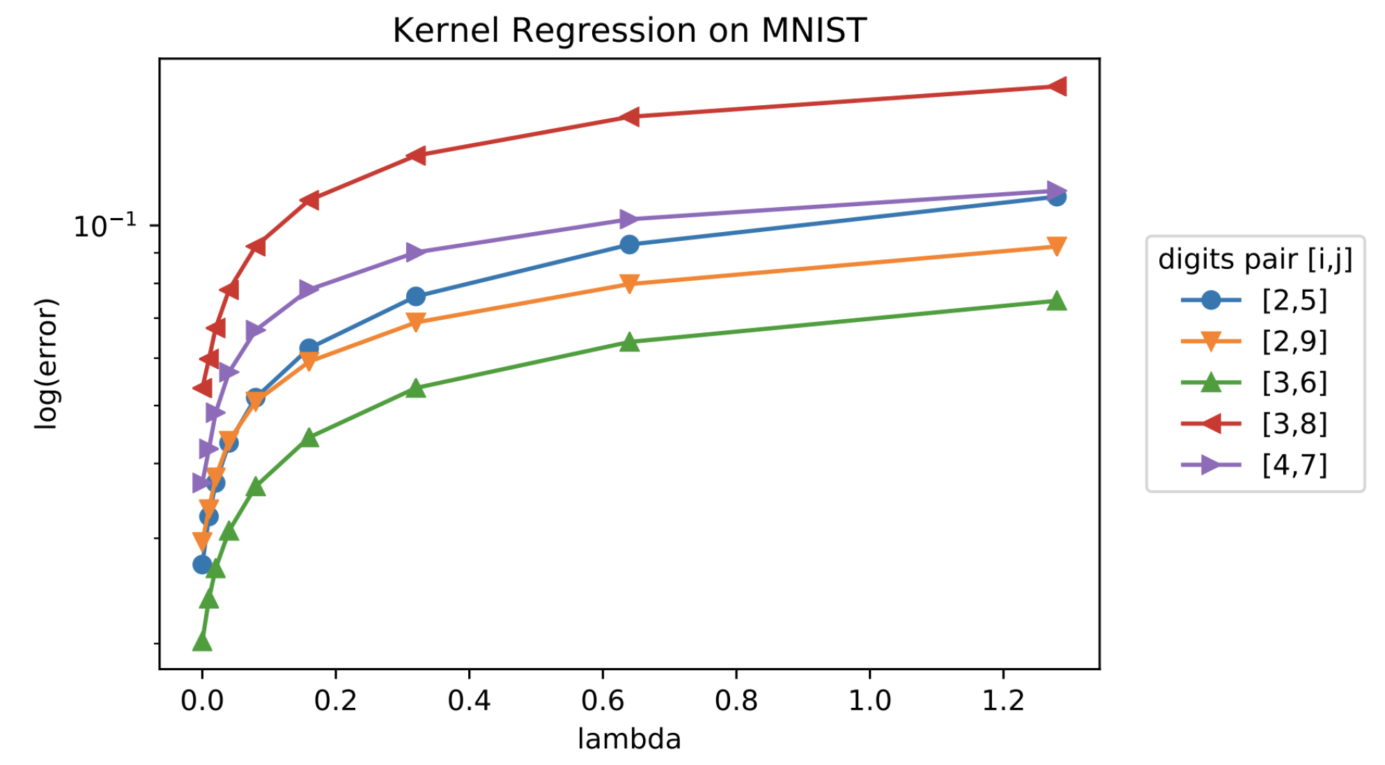
Fig 2. Test performance of Kernal ridge regression on MNIST digits for various values of regularization parameter $\lambda$

We can observe that on the contrary, the out-of-sample error is decreasing as we decrease the value of $\lambda$. Also, for virtually all pairs of digits, the best out-of-sample performance is achieved at $\lambda = 0$. This phenomenon is often called implicit regularization for interpolated minimum-norm solutions in Kernal ridge regression.

References

• Bartlett, Peter L and Mendelson, Shahar Rademacher and Gaussian complexities: Risk bounds and structural results JMLR 2002
• Chiyuan Zhang, Samy Bengio, Moritz Hardt, Benjamin Recht, Oril Vinyals Understanding Deep Learning Requires Rethinking Generalization ICLR 2017
• Mikhali Belkin, Alexander Rakhlin, Alexandra B Tsybakov Does Data Interpolation Contradict Statistical Optimality? PMLR 2019 Volume 89
• Mikhali Belkin, Siyuan Ma, Soumik Mandal To Understand Deep Learning We Need to Understand Kernel Learning PMLR 2018 Volume 80
• Mikhali Belkin, Daniel Hsu, Partha P Mitra Overfitting or Perfect Fitting? Risk Bounds for Classification and Regression Rules that Interpolate NIPS 2018
• Tengyuan Liang and Alexander Rakhlin Just Interpolate: Kernel “Ridgeless” Regression Can Generalize 2019